金融数据的交叉验证
传统验证方法在金融上为什么不行
像图像或表格数据,我们常用:
- K-fold cross-validation
- 随机划分训练/测试集
但是在金融(尤其是股市、币市)上:
价格数据是强时间相关的,而且分布随时间漂移(non-stationary)。
因此:
- ❌ 随机分割 → “未来数据”混进训练集(信息泄露)
- ❌ K-fold CV → 不符合时间因果
- ❌ 固定训练+测试划分 → 不能反映长期市场结构变化
这些都会让你的模型在训练集上表现很好,但实盘上全崩溃
在金融任务中,通常使用下列 3 种方法(越往下越贴近实盘)。
时间序列交叉验证 (TimeSeriesSplit)
优点:
- 简单易实现(
sklearn自带) - 不泄露未来信息
- 平衡“数据利用率”和“时序一致性”
使用场景:
- 模型结构、超参数调整阶段
- 适合验证模型的“平均泛化性能”
| 折数 | 训练数据 | 验证数据 |
|---|---|---|
| Fold1 | 1~100 | 101~150 |
| Fold2 | 1~150 | 151~200 |
| Fold3 | 1~200 | 201~250 |
滚动窗口验证 (Rolling Window Validation)
核心思想: 用固定长度窗口训练模型,然后滚动预测下一段时间。
优点:
- 模拟“定期 retrain 模型”的现实策略
- 反映模型对概念漂移 (Concept Drift) 的适应能力
示意图:
Train [1–100] → Predict [101–110]
Train [11–110] → Predict [111–120]
Train [21–120] → Predict [121–130]
特点:
- 窗口可以是固定长度(rolling)或扩展长度(expanding);
- 每次都重训模型;
- 非常适合高频交易或短周期预测。
Walk-Forward Validation (步进验证)
这是量化回测标准做法。
思路:
“在每个时点,只用已知历史训练模型,然后预测下一段时间。”
每次:
- 用过去数据训练;
- 预测未来;
- 滚动窗口前进;
- 累计所有预测,计算整体表现。
示意:
| 步 | 训练集 | 预测期 |
|---|---|---|
| 1 | 1–200 | 201–210 |
| 2 | 1–210 | 211–220 |
| 3 | 1–220 | 221–230 |
优点:
- 模拟真实交易中模型逐步更新;
- 无信息泄露;
- 适合回测策略;
- 可实时更新预测性能。
缺点:
- 计算量较大(每次都训练一个新模型);
- 实现稍复杂。
回测指标
仅仅看 MAE/MSE 不够。在金融中,更关心:
| 指标 | 含义 |
|---|---|
| Sharpe Ratio | 收益与风险比 |
| Max Drawdown | 最大回撤 |
| Hit Ratio / Accuracy | 方向预测正确率 |
| PnL(盈亏) | 模拟收益 |
| Calmar Ratio / Sortino | 回报稳定性 |
通常,我们会在 walk-forward 验证中:
- 模型预测未来一段收益方向;
- 构造简单交易策略;
- 回测计算上述指标;
- 得出真实金融表现。
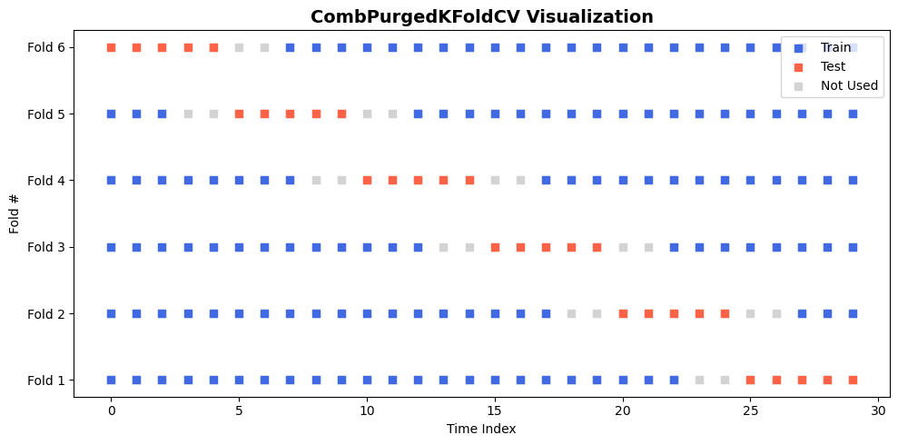
Purged & Embargoed Combinatorial Cross-Validation
这是 为金融时间序列设计的交叉验证方法, 专门用来:
- 防止 信息泄露 (Information Leakage),
- 防止 样本重叠 (Label Overlap),
- 在有时间依赖与事件窗口重叠的金融数据中,获得真实的泛化误差估计。
Purge(清除重叠样本)
- 删除所有训练样本中,
其
eval_time晚于测试集pred_time的样本。
这样训练集中不会包含与测试区间重叠的事件。
图示:
Train: |----A----|----B----|
Test:              |----C----|
Purge: 删除B(因为B的eval_time> C的pred_time)
Embargo(时间缓冲区)
- 在测试集结束后,再空出一段时间, 不让太近的训练样本参与。
这段“冷却时间”叫 embargo period。
目的:
避免由于样本间时间相关性,训练数据太靠近测试数据而污染结果。
图示:
Train: |----A----|         |----B----|
Test:             |----C----|
                   <---embargo period--->
这样模型不会看到测试后太近的数据。
Combinatorial Cross-Validation
它的 “Combinatorial” 是因为:
它不是像普通 K-fold 那样一次一个 test fold, 而是从 n 个折中组合出若干个可能的测试集组合。
比如:
- 10 折(n_splits=10);
- 每次选 2 折当测试(n_test_splits=2);
- 所有 45 种组合都会测试一次。
这比单纯 10 次交叉验证要更全面, 能更稳定地估计模型的“泛化分布”。
预测时间和评估时间
在金融时间序列(比如比特币价格)里, 我们训练模型时,每一条样本其实对应一个“事件”:
- 在 预测时间 (
pred_time) 我们看到了特征,模型做出决策; - 在 评估时间 (
eval_time) 我们才知道这次决策到底对不对。
比如:
我在 10:00 预测比特币未来 5 分钟会上涨; 到 10:05 才能知道结果是否真的上涨。
所以每一条样本不是一个点,而是一段时间区间:
[ pred_time , eval_time ]
预测时间(pred_time)
t1 = pd.Series(t1_).shift(time_gap)
shift(time_gap) 的意思是“往后推 200 个单位”,
比如:
| 原始时间索引 | 预测时间 (t1) |
|---|---|
| 0 | 200 |
| 1 | 201 |
| 2 | 202 |
也就是说:
样本 0 对应的预测时间是 200(往后看 200 个单位)。
👉 模型在时间 200 才会用样本 0 的信息来预测。
评估时间(eval_time)
t2 = pd.Series(t1_).shift(-time_gap)
shift(-time_gap) 是往前推 200 个单位。
| 原始时间索引 | 评估时间 (t2) |
|---|---|
| 0 | -200 |
| 1 | -199 |
| 2 | -198 |
| … | … |
也就是说:
样本 0 的预测结果在 -200 的时候已经能验证。
换句话说:
- 在
pred_time时刻,我们知道输入特征。 - 在
eval_time时刻,我们才知道“真相”能否评估预测是否正确。
举例 👇
样本 A:pred_time = 10:00,eval_time = 10:05
样本 B:pred_time = 10:03,eval_time = 10:08
→ 每个样本代表一个「事件窗口」 [pred_time, eval_time]。
时间泄露(information leakage)
假设我们在训练模型时用了样本 A, 而在测试模型时用了样本 B。
那问题是:
样本 A 的评估结果(eval_time = 10:05) 其实落在了样本 B 的预测时间(pred_time = 10:03)之后!
这意味着:
- 当模型在测试时(10:03)进行预测,
- 它的训练样本(10:05 才结束)包含了未来的信息(10:05 > 10:03)。
这在金融里是致命的未来信息泄露 (look-ahead bias)。
purging 的作用
为防止这种泄露,purge 规则是:
任何训练样本,只要它的 评估时间 (eval_time) 晚于任何测试样本的 预测时间 (pred_time),就要删除。
形式化表达: $$ \text{如果 } eval_time(train) \ge pred_time(test) \Rightarrow 删除该 train 样本 $$ 这样可以保证:
- 训练样本用到的数据都比测试样本更早;
- 没有交叉时间窗口;
- 模型验证结果更接近真实交易情形。
from CombPurgedKFoldCV import CombPurgedKFoldCV
import numpy as np
import matplotlib.pyplot as plt
N = 30
cv = CombPurgedKFoldCV(n_splits=6, n_test_splits=1, embargo_td=1, look_after=2)

fig, ax = plt.subplots(figsize=(10, 5))
ax.set_title("CombPurgedKFoldCV Visualization", fontsize=14, weight="bold")

# 每一折绘制一行时间条
for fold_idx, (train_idx, test_idx) in enumerate(cv.split(np.arange(N))):
    # 所有点背景置灰
    ax.scatter(np.arange(N), np.ones(N)*fold_idx, color="lightgray", s=40, marker="s", label=None)

    # 训练集蓝色
    ax.scatter(train_idx, np.ones(len(train_idx))*fold_idx, color="royalblue", s=40, marker="s", label=None)

    # 测试集红色
    ax.scatter(test_idx, np.ones(len(test_idx))*fold_idx, color="tomato", s=40, marker="s", label=None)

# 图例 & 样式
ax.set_yticks(range(fold_idx+1))
ax.set_yticklabels([f"Fold {i+1}" for i in range(fold_idx+1)])
ax.set_xlabel("Time Index")
ax.set_ylabel("Fold #")

# 图例样例
ax.scatter([], [], color="royalblue", s=40, marker="s", label="Train")
ax.scatter([], [], color="tomato", s=40, marker="s", label="Test")
ax.scatter([], [], color="lightgray", s=40, marker="s", label="Not Used")
ax.legend(loc="upper right")

plt.tight_layout()
plt.show()
代码
顶层架构概览
整个代码有三层:
┌────────────────────────────────────────────┐
│        BaseTimeSeriesCrossValidator        │  ← 抽象基类(模板)
├────────────────────────────────────────────┤
│        CombPurgedKFoldCV (子类实现)        │  ← 具体交叉验证逻辑
├────────────────────────────────────────────┤
│  purge() + embargo() + 辅助函数工具层      │  ← 时间安全性控制工具函数
└────────────────────────────────────────────┘
思路:
- 上层定义“接口规范与统一检查”;
- 中层定义“交叉验证的分割策略”;
- 下层定义“时间安全机制(purge + embargo)”。
下面是 BaseTimeSeriesCrossValidator
from abc import abstractmethod # 定义一种不能直接实例化、必须被继承实现的类
import pandas as pd

class BaseTimeSeriesCrossValidator:
    """
    抽象基类
    为所有时间序列验证器提供统一接口和输入验证逻辑。

    n_splits: 分成多少分, K-fold 的 K, >=2
    """
    def __init__(self, n_splits:int=10):
        self.n_splits = n_splits
        self.pred_times = None
        self.eval_times = None
        self.indices = None

    @abstractmethod
    def split(self, X: pd.DataFrame, y: pd.Series = None,
              pred_times: pd.Series = None, eval_times: pd.Series = None):
        pass
下面是 CombPurgedKFoldCV
from BaseTimeSeriesCrossValidator import BaseTimeSeriesCrossValidator
import numpy as np
import itertools as itt

class CombPurgedKFoldCV(BaseTimeSeriesCrossValidator):


    def __init__(self, n_splits = 10, n_test_splits=2, embargo_td=1, look_after=1):
        super().__init__(n_splits)
        self.n_test_splits = n_test_splits
        self.embargo_td = embargo_td
        self.look_after = look_after

    def split(self, X, y = None):
        self.indices = np.arange(X.shape[0])
        # 按时间顺序切分数据成多个折
        splited_indices = np.array_split(self.indices, self.n_splits)
        all_bounds = [[block[0], block[-1]+1] for block in splited_indices]
        # 枚举所有可能的测试组合
        bounds_selection = reversed(list(itt.combinations(all_bounds, self.n_test_splits)))
        for bounds in bounds_selection:
            test_indices, test_bounds = self.compute_test_set(bounds)
            train_indices = self.compute_train_set(test_indices, test_bounds)
            yield train_indices, test_indices

    def compute_test_set(self, bounds):
        # 如果相邻的测试折是连续的,就把它们合并成一个区间
        merged_bounds = []
        for x in bounds:
            if not merged_bounds or merged_bounds[-1][1] != x[0]:
                merged_bounds.append(x)
            else:
                merged_bounds[-1][1] = x[1]
        test_indices = np.array([], dtype=int)
        for l,r in merged_bounds:
            test_indices = np.concatenate((test_indices, self.indices[l:r]))
        return test_indices, merged_bounds

    def compute_train_set(self, test_indices, test_folds):
        train_indices = np.setdiff1d(self.indices, test_indices)
        for test_fold in test_folds:
            train_indices = self.purge(train_indices, test_fold[0])
            train_indices = self.embargo(train_indices, test_fold[1])
        return train_indices

    def purge(self, train_indices, test_fold_start):
        # 保证 train 的 eval_time < test 的 pred_time
        overlap = [i for i in train_indices if (i + self.look_after) >= test_fold_start and i < test_fold_start]
        train_indices = np.setdiff1d(train_indices, overlap)
        return train_indices

    def embargo(self, train_indices, test_fold_end):
        # test end 后一段时间不允许出现 train sample
        overlap = [i for i in train_indices if test_fold_end <= i <= test_fold_end + self.embargo_td]
        train_indices = np.setdiff1d(train_indices, overlap)
        return train_indices